LSTM CLASSIFICATION OF AUTOMATIC MODULATION CLASSIFICATION

Ben Ashby Steve Hauser Aditya Kashyap

Introduction

Neural networks have emerged as a tool for gathering insights from data that may be difficult or impossible for humans to deduce without computational assistance. Neural networks are often designed to generate function approximations between a set of input data and the desired output¹. One such scheme, the Recursive Neural Network (RNN), is well adapted to learn from sequential data in order to learn about relations between samples of the sequence². Our project uses a specific RNN, a Long Short-Term Memory (LSTM) network, to classify signals based on their modulation schemes. LSTMs have been used successfully in previous work³ to develop a method for early detection of motion templates. We liked the fact that the authors were able to detect motion sequences by merely looking at the first 24.77 frames on average (about 1 second) of a motion pattern. Hence we decide to use LSTMs and adapt them to our project.

The LSTM operates using two important concepts; cells and gates. Each cell (represented by a green block in the figure) contains three gates: an forget gate, the input gate, and the output gate⁴. The picture below⁵ provides a visual representation of the LSTM network. Click the image to view larger.

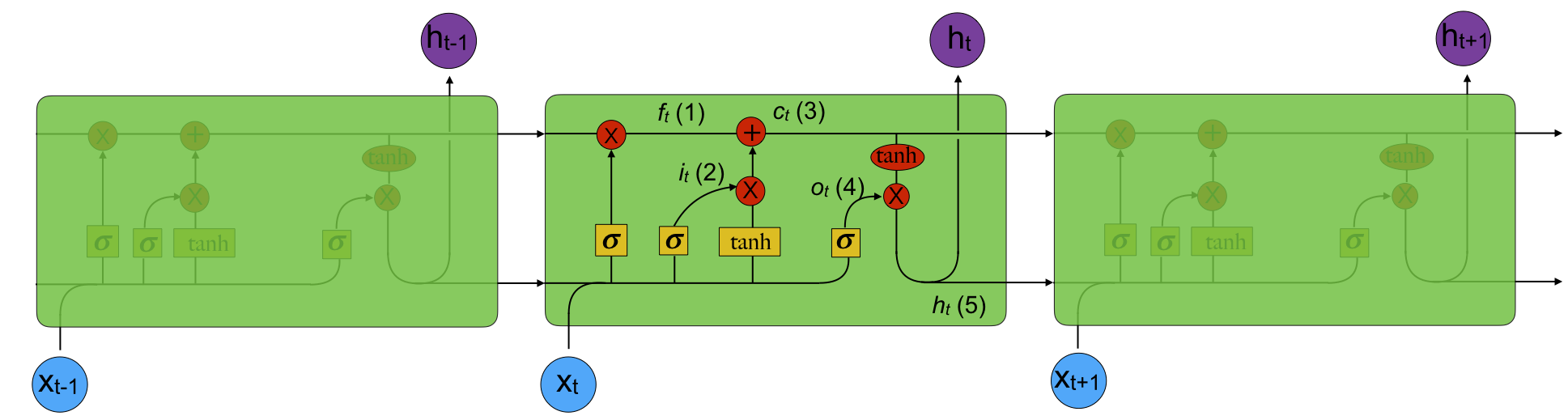
The forget gate is given by the equation:

(1) $\begin{align*}&f_t = \sigma (W_{xf}x_t + W_{hf}h_{t-1} + W_{cf}c_{t-1} + b_f)\end{align*}$

$\text{It takes in the input to the cell, } $x_t$, the output of the previous cell, $h_{t-1}$, and the output of the previous candidate layer, $c_{t-1}$ It applies weighting matrices $W_{xf}$, $W_{hf}$, $W_{cf}$ and bias factor $b_f$. Then it scales the components by a sigmoid function.$

The input gate is described by the equation:

(2) $\begin{align*}&i_t = \sigma (W_{xi}x_t + W_{hi}h_{t-1} + W_{ci}c_{t-1} + b_i)\end{align*}$

$\text{The equation takes }$x_t$, the input to the cell, $h_{t-1}$, the output from the previous cell, and $c_{t-1}$, the output of the previous candidate layer. It applies weighting matrices $W_{xi}$, $W_{hi}$, $W_{ci}$ and bias factor $b_i$. Then it scales the components through a sigmoid function.$

The candidate layer is computed using the equation:

(3) $\begin{align*}&c_t = f_tc_{t-1} + i_t \text{tanh}(W_{xc}x_t + W_{hc}h_{t-1} + b_c)\end{align*}$

It multiplies the forget gate value with the previous candidate layer value and sums it with the input value times the hyperbolic tangent of a linear combination of vectors.

The output gate and final output are given by the equations:

(4) $\begin{align*}&o_t = \sigma (W_{xo}x_t + W_{ho}h_{t-1} + W_{co}c_{t-1} + b_o)\end{align*}$

(5) $\begin{align*}&h_t = o_t \text{tanh}(c_t)\end{align*}$

$\text{The output gate } $o_t$ passes a linear combination of the input sample, the previous output value, and the previous candidate layer value through a sigmoid function. The output of the current cell, $h_t$, is the product of the output value and the hyperbolic tangent of the current cell's candidate layer.$

The network remembers its cell states between invocations, giving rise to the memory property of the network. Each gate has a weight matrix which defines the internal states.

Applications

The primary application of our work is in automatic modulation classification (AMC) for software defined radios. In general, software defined radios use a large variety of modulation schemes depending on the situation, and it can be helpful for a radio to be able to automatically determine the modulation of different signals without prior knowledge of the signals. For example, in spectral sensing applications, AMC can be applied to dynamically changing modulation formats, and can help identify primary vs. secondary users. Making a classification decision as early as possible can save valuable resources in a radio, and thus our project focuses specifically on early classification of time series data. Apart from cognitive radio, the concept of early classification on time series data can be extended to other fields such as in medicine to interpret ECG results and genomics, in financial markets, or in monitoring for abnormal behavior in computer systems⁶

Previous Work

A brief survey of sequence classification – Xing, Pei, Keogh 2010
This paper conducted a survey of the existing work on sequence classification. Their conclusion was that while there is a lot of work focused on simple symbolic sequences there is still more work to be done on multiple variate time series. They also concluded that early classification presents a challenge for future studies.

Early Classification of time series – Xing, Pei, Yu 2012
This paper formulated the problem of early classification of time series (ECTS). They proposed an ECTS classifier that showed comparable results to a 1NN classifier for the full time series. Their classifier works by finding the MPL(minimum prediction length) for a cluster of time series instead of a single time series.
However, they failed to provide a metric for calculating when we have seen enough of a signal to classify the signal and instead they plot the percentage accuracy for different prediction lengths.

Reliable early classification of time series – Anderson, Parrish, Tsukida, Gupta 2012
They developed an approach for early classification of signals using a generative classifier with a focus on quadratic discriminant analysis (QDA) classifier. They compare their method to the ECTS algorithm discussed in the paper above and it did seem to perform better.
They also provided a reliability bound but that is just the percent of examples that they got right for a given number of samples. So they plot a graph that shows the percentage that they classified correctly for n number of samples. However, when looking at one example, they fail to say if they have seen enough of that example to confidently classify it.

Classifying with confidence from incomplete information – Anderson, Parrish, Gupta, Hsiao 2013
In this paper the authors improve upon their work from 2012 by focusing more on the determining the reliability of the classification decision rather than just the class label. Their approach is to model the complete data as a random model whose distribution is dependent on the current incomplete data and the complete training data. The paper mentions optimal stopping rules but leaves it as a future work since it would require specification of misclassification cost and delay cost which the paper does not take into account and neither do we. The paper used three set of construction measures, the Chebyshev set, the Gaussian set and Naive Bayes box set and it used the GMM method for estimation. For us, the main take away was that their method, which had predictive power, performed better than the 1-NN and the local QDA methods in the earlier methods.
Our main takeaway from this paper was that we wanted a model that had some predictive power.We decided to look at more options and found a paper on LSTMs that seemed helpful. LSTMs have the advantage of modelling “memory” and hence we believed they too would inherently have the advantage of predictive power.

This paper does not use LSTMs for time series signals like we want to but rather for Early Recognition of Motion patterns but it was still helpful to get an idea of how to use LSTMs for Early Recognition.

LSTM-Based Early Recognition of Motion Patterns – Weber, Liwicki, Stricker, Scholzel, Uchida
This paper presented a method for early detection of motion templates. They developed an algorithm to provide recognition results before a motion sequence is completed. Though we were not working on motion sequence, the general idea of training on a data set and using that to classify test data even before seeing it in its entirety was useful to us. The authors achieved 88% accuracy with LSTMs. Furthermore they were able to classify a motion pattern in merely one second which is an excellent result.

Methodology

Our training and testing datasets were synthetically generated to simulate 8 different modulation schemes: 2FSK, 4FSK, 8FSK, BPSK, QPSK, 8PSK, 16QAM, and 64QAM. Based on previous works, we decided to use an LSTM network. Intuitively, this makes sense because those networks are designed to learn from a stream of data, such as the time series IQ values we are using.

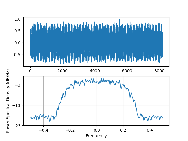
Below is a sample of one of the modulation schemes, just to give a sense of the input data. The top plot is the raw IQ time series, and the bottom plot is the power spectral density of the signal.

The neural network was built and trained using Keras and TensorFlow. A simple network was build using a single layer LSTM with 256 cells followed by an 8 node fully connected layer. The fully connected layer used the softmax function to classify between 8 different class types. The LSTM used a tanh activation function and a hard sigmoid for the recurrent activation. While the LSTM can make decisions after an arbitrary number of samples, we elected to stop training after 512 samples. Additionally, because the input data was a complex valued, raw IQ stream, the input was reformatted to be of size (512, 2) so that the real and imaginary components were treated as “features” of the input data. Training took approximately 3 days on a standard workstation. We trained using 800,000 samples, tested using 160,000 examples, and validated using 80,000 samples. To avoid overfitting, classification accuracy on the validation dataset was constantly monitored, and when it stopped improving training was terminated. The final trained network had an overall classification accuracy of about 83% on the test dataset.

Proposed Solution

Our goal was to find a metric for early classification of the modulation schemes, as simply detecting the scheme itself is not very useful if it takes a long time to arrive at an accurate answer. Therefore, we investigated 2 methods to minimize the number of samples needed while still attaining a reasonable level of accuracy in our guess. The first was using a softmax function to produce a probability-like output for the best guess. This had limited success, so we also tried praying to Apollo and Athena in the hopes that they would bring divine intervention into the process.

Divine intervention brought us towards using a window size and threshold values.

Once we found a solution, our goal was to experimentally prove that the early stopping criteria was bounded for all the modulation schemes, or at least a subset of them.

Results and Anaylsis

Results From Raw Softmax Output

The first plot seen below shows the network was able to classify the signal after only a few samples. This plot motivated us to further investigate early classification since it works in some cases, but we wanted to understand when early classification was a viable option.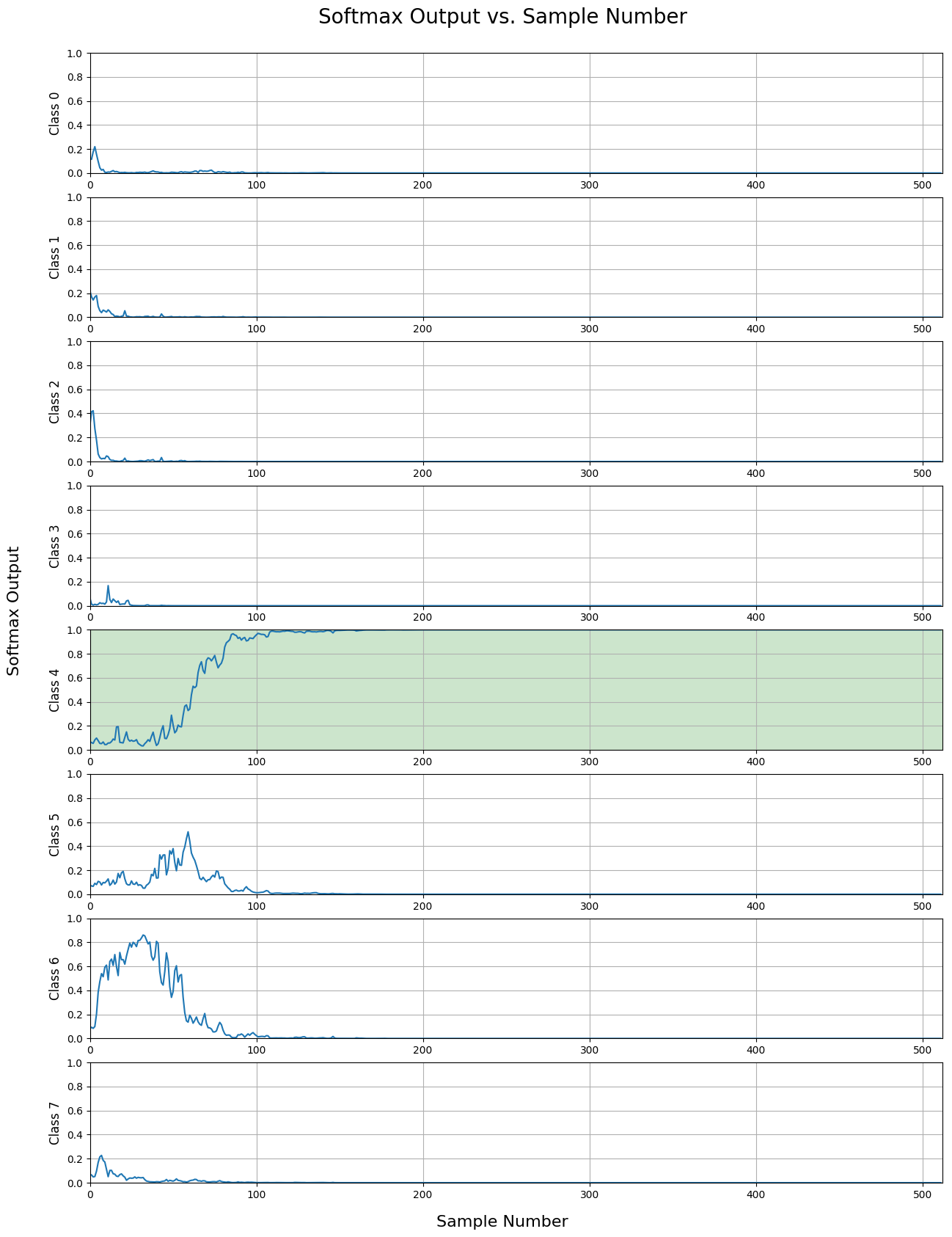

The next plot shows an instance when if the signal were classified too early, it would have made an error since an incorrect signal has a high output initially. Only later does the network find the correct classification.

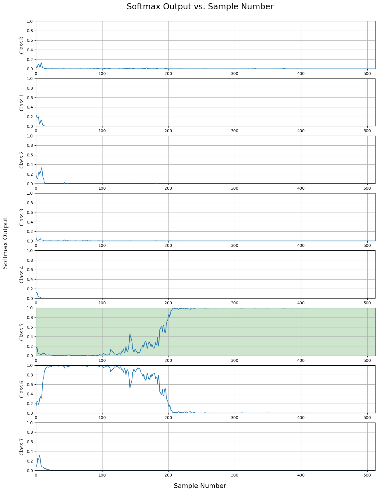
The third plot shows a signal that wasn’t classified until the very end of the sample stream, and not by a large margin. From this data, one can see that the network can find it difficult to make the correct decision in a timely manner.

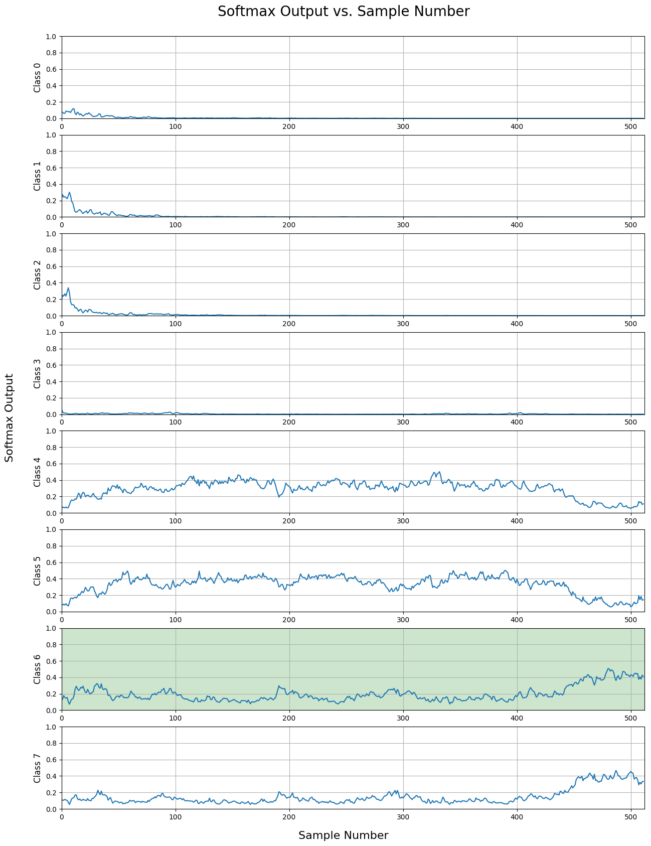
The final plot below shows when the network was unable to make a correct decision from the sample stream. This shows that the network can fail to make the correct classification at times.

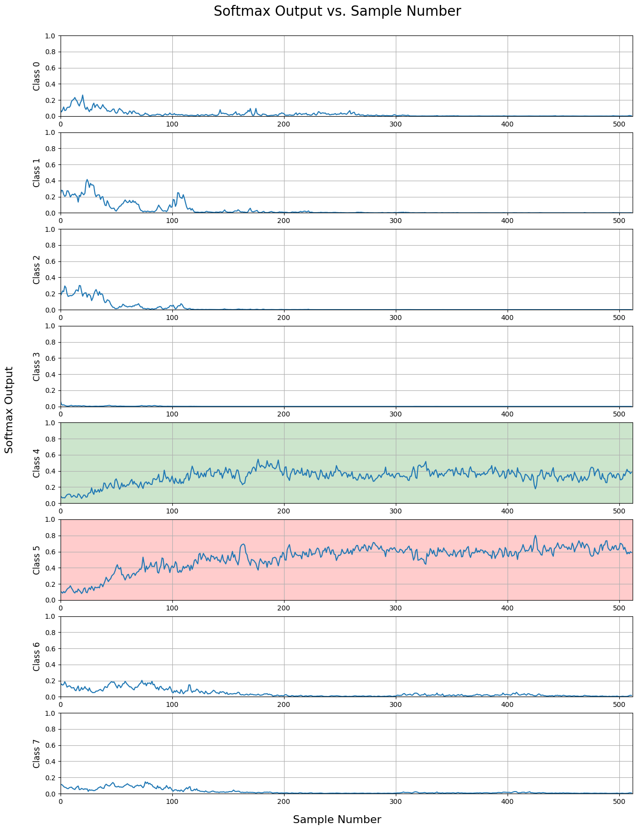
Looking at these inputs suggested that this might be a good case for early classification.

The next two graphs demonstrate the effect of noisy signals on classification, and overall accuracy of classification as a function of the number of samples. In the first plot, low SNRs adversely effect the network’s ability to classify correctly. An SNR of about 10 or higher is desirable. As for number of samples, the first plot shows that there is a large advantage to increasing the sample size until about 192 samples, at which point there are diminishing returns on further increasing the sample size.

The second plot gives a more general overview of overall classification accuracy as a function of number of samples used. Likewise, there are diminishing returns with increasing the number of samples used to classify past a certain point.

From these graphs, we can gather that an SNR of about 10 or higher and about 150-200 samples are required for a decent classification accuracy.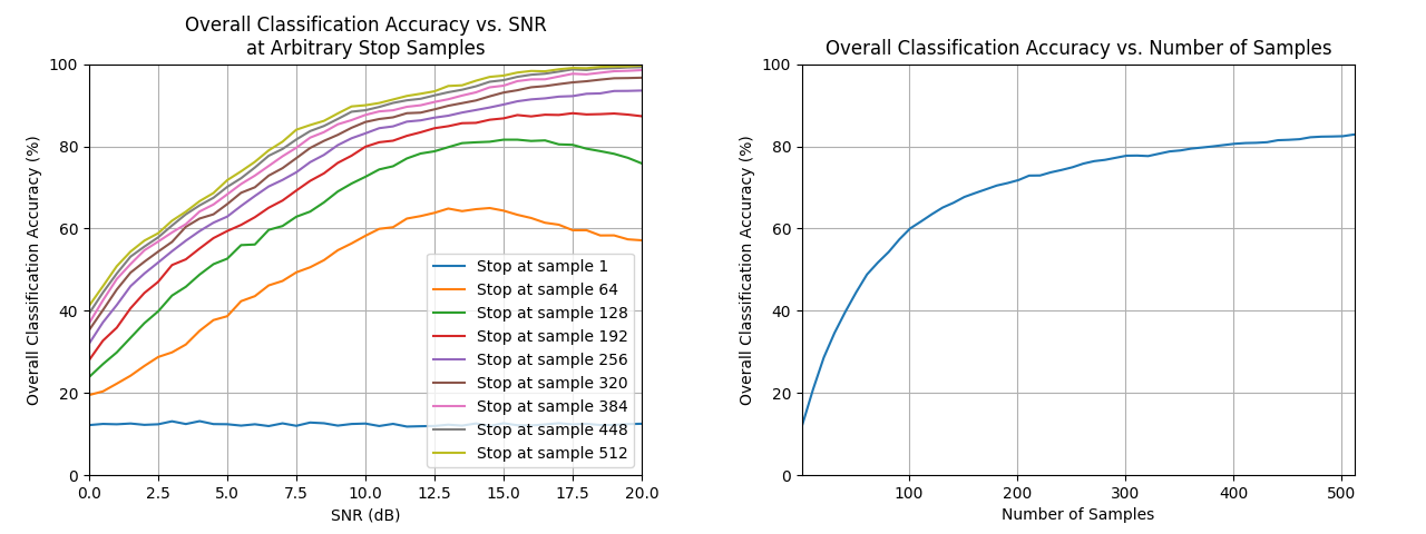

From these, we concluded that pursuing an early classification scheme may be viable, and our next step was to find a softmax early decision boundary.

The next step was to investigate if we could find a softmax decision threshold that would optimize the classification accuracy while keeping the number of samples to a minimum.

The first plot shows that as the decision threshold is increased, the accuracy of the classification also increases. However, the trade-off is the network’s early classification capability is impaired. Here, early is defined as any time before the 512 sample size.

The second plot shows on average, how many samples are required to make a classification as a function of the softmax decision boundary. Note that as the decision boundary increases, more samples are required before a decision can be reached, and about 300 samples are required before the network is sufficiently accurate in its decisions. Past 300 samples, there is little to gain from using more since the sample size to increased decision boundary trade-off is low.

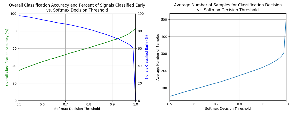
To get accuracy of about 75%, we need a softmax decision boundary of about .95. But from second graph, the average number samples required for .95 is about 275, or half the samples. To further increase the accuracy from 75% to 80%, we must make decision threshold almost .99. At that point, we have to look at nearly the entirety of the 512 samples, so there is no advantage to using the softmax decision threshold for early classification.

Stability Metric™

The next solution we developed was a classification stability metric, which is comprised of a window and a tolerance factor. The window width is set to a certain number of samples, during which we check if the softmax outputs for the sample changes in that time span. The amount of change allowable is set by the tolerance factor. If the change is too great, then the network continues to classify more samples.

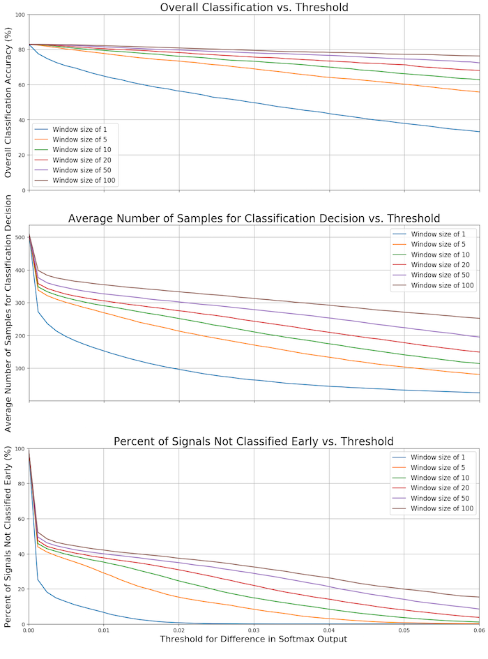
The plot below shows this metric provides significantly better results than the softmax decision boundary. All three plots have threshold for difference in softmax decision output on the x-axis.

The top plot shows the relation between overall classification accuracy as a function of difference in decision thresholds for various window sizes. There is a diminishing return with choosing larger windows, in that at tight tolerance levels, you don’t see much improvement in accuracy. Also, note that as your tolerance gets looser, the classification accuracy decreases.

The middle plot shows the average number of samples required to make a classification decision as a function of the tolerance factor. This gives us a sense of how soon we can make a classification using the tolerance factor and window size metrics. If the tolerance is too low, then it takes a large number of samples. Intuitively this makes sense, because we never recognize that we’ve stabilized to a classification decision.

The bottom plot shows the percentage of signals that were not classified early for various window sizes of a range of tolerances. Again, if the tolerance is too tight, we cannot make a decision early in the sample stream.

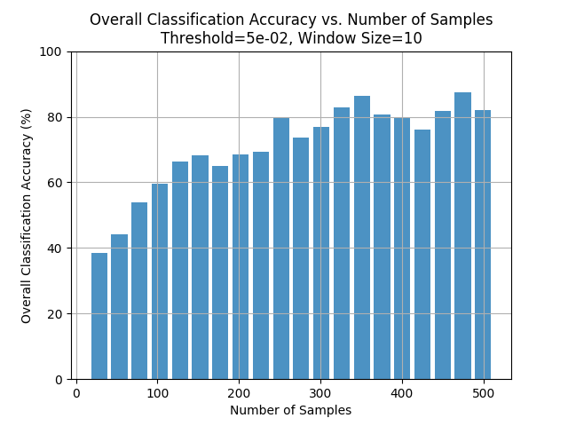
Adjusting Window and Tolerance Sizes

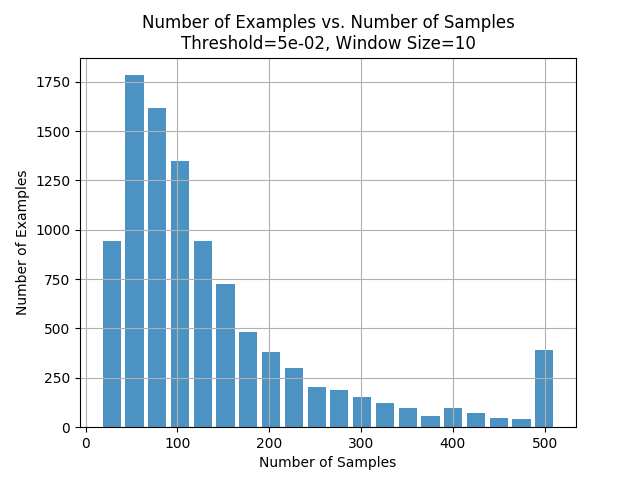
This graph shows us the number of samples that got classified after looking at n number of samples. We plot this for a window size of 10 and tolerance of 0.05 which are the parameter values we find to be optimal.
We see here that for most of the examples, we need only 100 samples or fewer before making a decision which is encouraging.

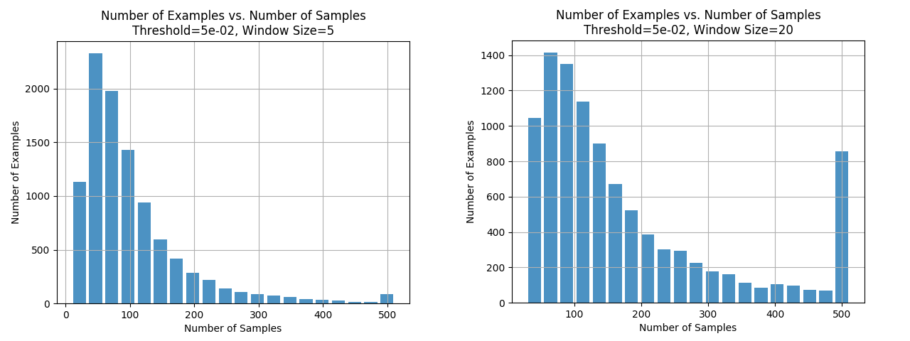
To justify our choice of parameter values we see what happens when we change the window size and tolerance

For a window size of 5, we see that as we decrease the window size, we need even fewer samples to make a decision. While this seems to be what we want, we have to remember that we’ve seen earlier that the accuracy fell when we switched to a window size of 10.

We saw earlier that increasing the window size provides greater accuracy. However, a greater window size also requires the majority of samples before a decision is made. An early decision is not possible in this case.

As expected, these two graphs, emphasize the trade off we have seen been accuracy, window size and early classification.
To us, a window size of 10 seemed like a good balance with most of the signals being classified early with acceptable accuracy.

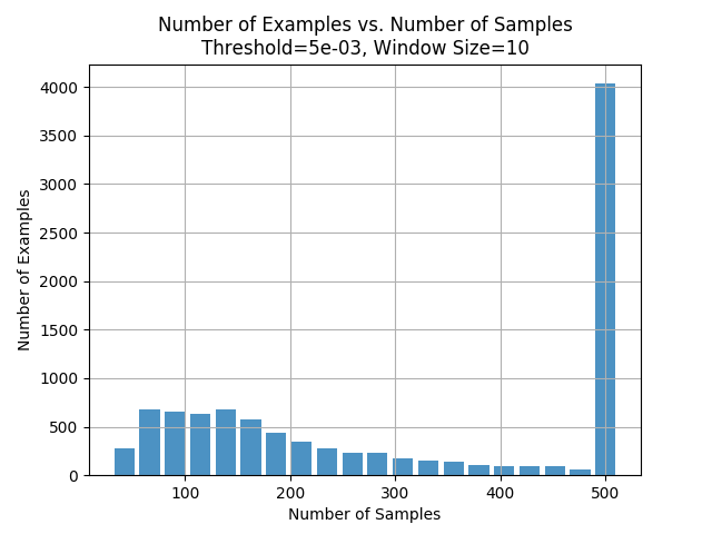
Here we see that if we are too strict about the tolerance, we can never make a decision about which class the signal belongs to because the softmax outputs don’t stabilize enough and as a result we make very few early classifications.

This plot shows us that the accuracy is about 60% for the signals for which we see about 100 samples. We also note that that there isn’t really a sharp jump in accuracy by seeing more samples and we hit a point of diminishing returns.
Also, recall that with our window size of 10 and tolerance of 0.05, we were only seeing about 100 samples for most cases. This gives us an idea on what we could do to improve upon our work in the future. We could look at at least 100 samples before we make a decision.

Conclusion and Suggestions for Future Work

While early classification remains an open problem, we hope that we have made a useful contribution to the field. This project showed that early classification using LSTM neural networks might be practical for AMC, and that reliable metrics can be determined and easily applied. While this project focused specifically on AMC using raw IQ samples, we expect that the metrics developed here would apply to any time-series data. In future work exploring more sophisticated metrics such as enforcing a lower bound on the required number of samples in conjunction with our stability metric, or dynamically changing the metric based on SNR may further improve the early classification performance.

Accompanying Video

Bibliography

[1] Goodfellow. Deep Learning. MIT Press, 2016.
[2] S. Hochreiter and J. Schmidhuber. Long short-term memory. Neural Computation, 9(8):1735–1780, 1997.
[3] LSTM-Based Early Recognition of Motion Patterns – Weber, Liwicki, Stricker, Scholzel, Uchida
[4] N. Pant. A guide for time series prediction using recurrent neural networks (lstms), Sept. 2017.
[5] C. Olah Understanding LSTM Networks, Aug. 2015
[6] Xing, Z., Pei, J. & Yu, P.S. Knowl Inf Syst (2012) 31: 105. Early Classification of time series

One Day at a Time